Coin flipping with a continuous prior

Coin flipping with a continuous prior#

In this example, we revisit the coin flipping example but now we will consider a continuous distribution for the \(\theta\) parameter. This will require us to use a different approach.

1. Model formulation#

Same as before, our model has two random variables, but we will make some simplifications. The number of tosses in specified in advance \(\#tosses\), so that for one experiment we only have to specify the number of heads:

\(\#heads\): random variable representing the number of heads in a sequence of coin tosses.

\(\theta\): probability of getting a head

The probability of a particular experiment outcome is given by the binomila distribution:

\[ \begin{align} P(\#heads\ |\ \theta) &= \binom{\#tosses}{\#heads} \theta^{\#heads}(1 - \theta)^{\#tosses - \#heads} \end{align} \]

This term is called the likelihood, the conditional probability of the data given the parameters.

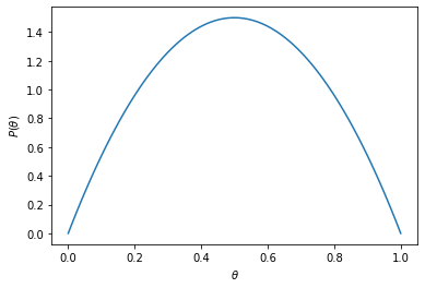
For modeling the prior we will use a beta distribution.

\[ P(\theta) = \text{Beta}(2,2) \]

The following code plots the prior with the help of TF Probability

import tensorflow_probability as tfp
tfd =  tfp.distributions

import numpy as np
import matplotlib.pyplot as plt


def theta_prior_fun():
    return tfd.Beta(2,2).prob

    
theta_prior = theta_prior_fun()
theta_vals = np.linspace(0, 1, 100)
theta_p = [theta_prior(val) for val in theta_vals]
ax = plt.subplot()
plt.plot(theta_vals, theta_p)
ax.set_xlabel(r'$\theta$')
ax.set_ylabel(r'$P(\theta$)');

../_images/a7a30d578152fcb672156ff19d7e84be9e1320f53352ceba691c6dbd0f92a262.png

Instead of modeling the prior and the likelihood separately, we will model them jointly. Remember that:

\[ P(\#heads, \theta) = P(\#heads | \theta)P( \theta) \]

So, we will use tfd.JointDistributionSequential to model this joint probability. JointDistributionSequential allows us to specify the dependencies among our random variables along with their corresponding distributions.

def create_joint_distribution(num_tosses):
    joint = tfd.JointDistributionSequential([
                       tfd.Beta(2, 2),                                   # theta
        lambda  theta: tfd.Binomial(total_count=num_tosses, probs=theta) # num_heads
    ], batch_ndims=0) #, use_vectorized_map=True)
    return joint

We can use a JointDistributionSequential object to draw samples from the joint probability distribution, as well as for calculating the unnomarlized probability of a sample.

# Creates a joint distribution object for 10 tosses
jd = create_joint_distribution(10) 

# Draws 5 samples
sample = jd.sample(5)

print(f'Theta vals:{sample[0].numpy()}')
print(f'#heads vals:{sample[0].numpy()}')

# Calculate the log probability of this samples
prob = jd.log_prob(sample)
print(f'Log probabilities:{prob.numpy()}')

# Draws a plot of the joint probability for #heads = 6

WARNING:tensorflow:@custom_gradient grad_fn has 'variables' in signature, but no ResourceVariables were used on the forward pass.
WARNING:tensorflow:@custom_gradient grad_fn has 'variables' in signature, but no ResourceVariables were used on the forward pass.
Theta vals:[0.5571841  0.2368055  0.56320196 0.15977305 0.7668681 ]
#heads vals:[0.5571841  0.2368055  0.56320196 0.15977305 0.7668681 ]
Log probabilities:[-1.487639  -1.4891112 -1.0213742 -1.4703302 -1.3688765]

2. Data collection#

Two collect data we can toss a real coin a number of times and record how many heads (\(\# heads\)) and tails (\(\# tails\)) we get. This is our data \(D\). For this exercise let’s assume we got \(\# heads = 15\) out of \(\#tosses = 20\).

3. Posterior calculation#

Instead of calculating explicitely the posterior (\(P(\theta|\#heads)\)) we will draw samples from it with the help of a MCMC sampler. To do so we need to first define the target log probability function. This function will depend only on \(\theta\) which is the variable that we will sample.

num_tosses = 20
jd = create_joint_distribution(num_tosses) 

num_heads = np.array([15])

def target_log_prob_fn(theta):
  """Unnormalized target density as a function of states."""
  return jd.log_prob((
      theta, num_heads))

It is important to remember that we are modeling the joint probability \(P(\#heads,\theta)\) which is proportional to \(P(\theta|\#heads)\) since:

\[ P(\theta|\#heads) = \frac{P(\#heads,\theta)}{P(\#heads)} \]

We can think of the joint as an unnormalized posterior. Let’s plot this unnormalized posterior for different values of \(theta\), to get an idea of how the real posterior looks like:

theta_vals = np.linspace(0, 1, 100)
theta_unnorm_posterior = [np.exp(target_log_prob_fn(val)) for val in theta_vals]
ax = plt.subplot()
plt.plot(theta_vals, theta_unnorm_posterior)
ax.set_xlabel(r'$\theta$')
ax.set_ylabel(r'$P(\theta,$#heads$=15})$)');

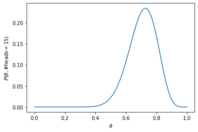
../_images/7589cf4fed5553246f794403653d23d40748ba019f66163c3a5b14a29ea2c1fa.png

Notice that the distribution is skewed towards the right.

Now we can draw samples with the help of MCMC

num_results = 50000
num_burnin_steps = 3000

# Improve performance by tracing the sampler using `tf.function`
# and compiling it using XLA.
@tf.function(autograph=False, jit_compile=True)
def do_sampling():
  return tfp.mcmc.sample_chain(
      num_results=num_results,
      num_burnin_steps=num_burnin_steps,
      current_state=[
          tf.constant([0.5], name='init_avg_effect'),
      ],
      kernel=tfp.mcmc.HamiltonianMonteCarlo(
          target_log_prob_fn=target_log_prob_fn,
          step_size=0.05,
          num_leapfrog_steps=3))

states, kernel_results = do_sampling()
num_accepted = np.sum(kernel_results.is_accepted)
print('Acceptance rate: {}'.format(num_accepted / num_results))

/usr/local/lib/python3.7/dist-packages/tensorflow_probability/python/mcmc/sample.py:339: UserWarning: Tracing all kernel results by default is deprecated. Set the `trace_fn` argument to None (the future default value) or an explicit callback that traces the values you are interested in.
  warnings.warn('Tracing all kernel results by default is deprecated. Set '

Acceptance rate: 0.9743

Now we can plot a histogram of the obtained samples, that can be used as an empirical distribution.

plt.hist(states[0].numpy(), bins=100);

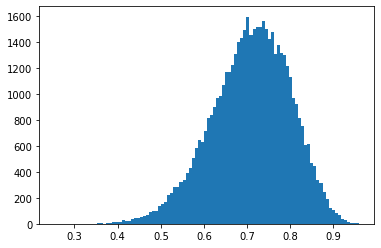
../_images/0f929b592f517809f6e58d21267c5e11a3526aa38bc9c3c858ad591740b7664e.png

Now we call the function with our data and plot the resulting posterior distribution:

4. Model application#

We can use the set of samples, \(\{\theta_i\}_{i=1\dots N}\), to calculate summarizations of the posterior distribution. For instance to calculate the Bayes estimators, we can approximate it by averaging the samples:

\[ \theta_{\text{Bayes}} = E[\theta] \approx \frac{1}{N}\sum_{i=1}^N \theta_i \]

def bayes_estimator(samples):
    return np.average(samples)

print(f'Bayes estimator:{bayes_estimator(states[0].numpy())}')

Bayes estimator:0.708452582359314